AN10073 How to Setup a Real-time Oscilloscope to Measure Jitter

Content

1. Introduction
2. Step 1: Initialize the instrument
3. Step 2: Optimize the vertical resolution
4. Step 3: Optimize the sampling rate
5. Step 4: Optimize the oscilloscope bandwidth
6. Step 5: Optimize the threshold voltage
7. Step 6: Select a type of jitter to measure
8. Step 7: Select a jitter filter
9. Step 8: Optimize the memory depth
10. Related Resources

1. Introduction

One of the most common instruments used to measure jitter is the real-time digital oscilloscope (scope). Real-time oscilloscopes must be configured properly to make accurate jitter measurements. This application note provides general guidelines to set up an oscilloscope for best jitter measurement accuracy.

The digital scope uses an internal time base to sample its inputs at regular intervals. The sampling rate can range from 1 Gsps (giga-samples-per-second) to 256 Gsps for the high-end units. Figure 1 illustrates how the scope samples and displays a signal presented to its inputs. The arrows at the bottom of the figure represent the sampling points, the solid line is the actual signal, and the dots are the sampled values. The signal displayed by the scope (represented by the dotted line) is the best-fit curve across the sampled points.

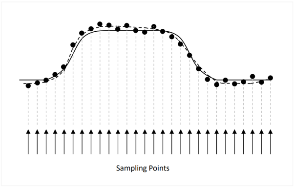
Figure 1. Sampling of a signal by a digital scope

The reader may notice that the sampled values do not always match that of the actual signal. These discrepancies are caused by errors in the scope. Most of these errors are inherent in the design/cost tradeoffs of the scope but proper scope setup can mitigate some of these inaccuracies. For example, the sampling points in a digital scope are generated by an internal time base. As a clock source, the time base has its own jitter characteristics, which contribute to the jitter measurement error. In general, time base jitter should be kept below 25% of the of the expected signal jitter to support jitter measurement with better than 3% accuracy. SiTime recommends using the best scope available to perform jitter measurements because higher-end units tend to have better time base circuits with lower jitter.

Use the following step-by-step procedure to manually setup the instrument for measuring jitter of all types for any real-time oscilloscope, regardless of manufacturer. Although specialized jitter-analysis software can be purchased from the manufacturer to auto-configure the instrument using a one-button or wizard-type approach, the software doesn't always produce the optimum configuration. Autoconfigured setups should therefore be verified using the same procedure (below). To configure the instrument for best jitter accuracy, perform the following steps in order.

2. Step 1: Initialize the instrument

Turn on the oscilloscope and restore the factory default setting. Then adjust the following items and save the measurement configuration for easy recall in the future.

• Set the oscilloscope mode to real time.
• Set the input termination to be 50 Ohms.
• Disable waveform averaging.
• Remove any delay between the first sample point and the trigger event. This reduces error from timebase instability.
• Configure the measurement setup to analyze all data acquired, rather than a subset of data.
• Select a relatively large record length (memory depth) so that a significant population of jitter data can be measured. Instructions for optimizing are below.
• Select the highest sampling rate. Instructions for optimizing are below.
• Select the highest oscilloscope bandwidth available. Instructions for optimizing are below.

3. Step 2: Optimize the vertical resolution

High-speed oscilloscopes typically employ analog-to-digital converters (ADCs) with at least 8 bits (256 levels) of quantization. The voltage reported by the ADC equals the true signal voltage plus a quantization error. This error is essentially a rounding error, so to minimize it, we need to reduce the voltage range captured by each quantization level. We do this by reducing the vertical resolution, or volts-per-division, setting. The goal is to use the full range of the ADC. For most oscilloscopes, this means adjusting the signal waveform until it just fills the vertical height of the display. Some oscilloscopes, however, are designed to overfill the display slightly to utilize an extra bit in the ADC to digitize the signal (contact the scope manufacturer to learn more). Make sure not to saturate the ADC, since this will destroy the integrity of the waveform.

Figure 2 shows how the jitter measurements improve by simply reducing the vertical resolution from (a) 100 mV/div to (b) 54 mV/div for an example 36 MHz clock signal, and 3 types of jitter: time-interval error (TIE), period jitter, and cycle-to-cycle (C2C) jitter, reported in units of seconds peak-to-peak (pp) and root-mean square (RMS). For reference, Figure 2(a) shows the auto-scaled signal, which, incidentally, should never be used to measure jitter.

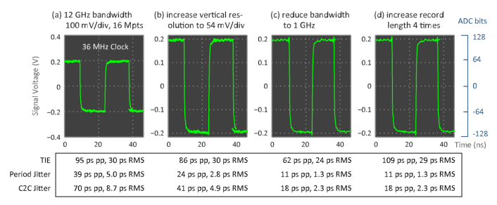
Figure 2: Illustration of jitter measurements in a 36 MHz clock signal using (a) auto-scaled settings, followed by (b) optimizing the vertical resolution, (c) optimizing the system bandwidth, then observing the effect of (d) increasing the record length

4. Step 3: Optimize the sampling rate

In theory, the sampling rate must be at least two times the highest analog frequency present in the signal to avoid aliasing. In practice, the acquisition process requires oscilloscopes to sample at 2.5 to 3 times this frequency. A conservative rule of thumb is to set the sampling rate so that each edge is sampled at least 5 times. More is always better to minimize interpolation error when computing jitter. The downside to higher sampling rates is a smaller population of jitter measurements, unless the memory depth can be increased.

If the edge cannot be sampled at least 5 times using the highest sampling rate provided by the oscilloscope, try to obtain at least 3 sampling points between the 20% and 80% points of a rising and falling signal, respectively. For example, if the rise time (20% - 80%) of a signal is 1 ns and 4 sampling points are needed within this time frame, then the scope must have a sampling rate better than 4 Gsps. If the scope has a higher sampling rate, select the highest sampling setting. Finally, sinc interpolation can be enabled to provide additional data points, at the expense of processing time.

5. Step 4: Optimize the oscilloscope bandwidth

The inputs to a digital scope passed through an analog amplifier before they are digitized by the analogto-digital converter (ADC). The noise produced by this amplifier is proportional to the input bandwidth of the scope: the wider the bandwidth, the higher the noise. However, reducing the bandwidth too much will affect the rising and fall time of the sampled signal, thus introducing significant errors to the jitter measurement.

The general equation describing the relationship between rise time/fall time and the bandwidth of the signal edge is:

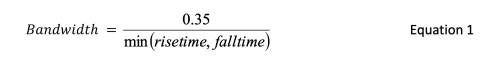
where the rise time (or fall time) is measured between the 20% and the 80% points of the signal edge. A common rule of thumb for measuring NRZ data is to set the bandwidth of the oscilloscope (plus probes if used) to at least 1.8, and more preferably 2.8, times the bit rate. When measuring clock signals with analog output-voltage levels, set the bandwidth to capture at least the 5th harmonic. Clock signals with digital levels have significant spectral energy at much higher harmonics, and a bandwidth of 20 to 30 times the fundamental frequency is recommended. In some scopes, the bandwidth can be set only if the maximum sampling rate is selected. In other scopes, the bandwidth may not be selectable at all.

One method to set the optimum bandwidth in just a few seconds is to measure the rise time at the highest bandwidth, then lower the bandwidth until just before the rise time changes more than 5% from its highest-bandwidth value. Figure 3 illustrates such an experiment for an oscilloscope having a maximum analog bandwidth of 12 GHz. The y-axis is the rise (and fall) time normalized to the value at 12 GHz and expressed as a percentage. The optimum bandwidth is observed to be 1 GHz. Using a higher bandwidth would raise the instrument's jitter noise floor; using a lower bandwidth would slow the measured edges down and increase jitter from AM to PM conversion. Figure 2(c) shows how the jitter values improve by reducing the acquisition bandwidth from 12 GHz to 1 GHz, which results in a lower instrument noise floor.

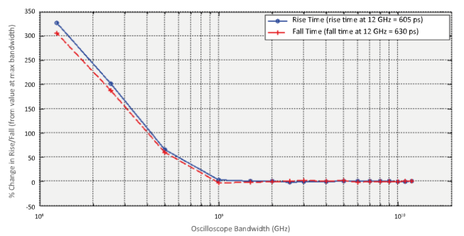
Figure 3: This plot shows how a 36 MHz clock (shown in Figure 2) rise and fall times change as the oscilloscope bandwidth deviates from 12 GHz. The rise and fall times are fairly constant moving from 12 GHz to a 1 GHz bandwidth, then increase rapidly for lower bandwidths. The optimum oscilloscope bandwidth for this device is therefore 1 GHz.

6. Step 5: Optimize the threshold voltage

The threshold voltage is the vertical level used by the oscilloscope to determine where to measure jitter. Ideally this level is set to emulate the level used by receiver circuitry in an end application. The threshold voltage is the voltage level that causes the decision-threshold circuit in a receiver to change state when the input signal crosses it. For example, the threshold voltage for a differential signal is 0 V. The oscilloscope uses the closest sampled points on either side of this threshold to interpolate a crossing point at the threshold voltage, which is then used to measure jitter.

Set the threshold voltage as an absolute voltage, rather than as a percentage of the voltage swing. Figure 4 illustrates why. If the waveform (a) is amplitude modulated, (b) does not settle at logic high (or logic low), or (c) contains ringing or other artifacts, the 50% level (red markers in Figure 4) of the amplitude swing can vary or be offset from the level that a reference receiver (gray lines in Figure 4) would observe in a system.

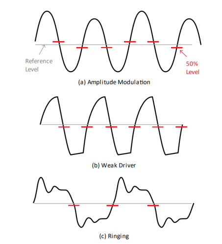
Figure 4: For accurate jitter measurements, set the threshold voltage at an absolute level (gray line), rather than at 50% of the swing (red markers)

The hysteresis voltage (sometimes specified as upper and lower voltage thresholds) will also need to be set to prevent detecting false edges, which can occur if noise in the signal causes the threshold voltage to be crossed multiple times per edge. Set the hysteresis voltage slightly larger than the maximum voltage spike expected in the signal. The voltage can be estimated with an oscilloscope measurement. Simply setup the scope according to all the steps in this procedure (including all steps above and below), then either turn off the DUT's power or disconnect the DUT from the oscilloscope. Capture a waveform, then measure the maximum peak-peak voltage over the entire waveform. Add a little margin to this value and use it to compute a hysteresis value that can be entered into the oscilloscope (e.g., either peak, or peak-peak, as appropriate for the particular oscilloscope in use). Typically the default hysteresis setting is sufficient, unless the signal is very noisy.

7. Step 6: Select a type of jitter to measure

Set the type of jitter to measure (TIE, period jitter, C2C jitter, etc.), along with the edges of interest (e.g., rising edges only, falling edges only, or all edges).

8. Step 7: Select a jitter filter

Optionally, software filters can also be applied to the measured jitter values to model a system's response to a signal passing through it. The goal of the filter is to extract only the jitter that would be observed by the real system. For example, TIE is always filtered as required by high-speed serial standards. When applicable, set the filter characteristics according to an industry standard or system requirement.

9. Step 8: Optimize the memory depth

Note that the oscilloscope itself acts as a brick-wall bandpass jitter filter. The upper (low-pass) corner frequency is set by the oscilloscope bandwidth. The lower (high-pass) corner frequency equals 1 divided by the acquisition time. In other words, the lower corner frequency equals the sample rate divided by the record length, where the record length is the number of samples acquired.

The lower corner frequency deserves special attention since it can greatly affect the measured jitter values. Suppose we acquire a jitter-free signal as shown by the blue curve in the bottom of Figure 5.

Next add phase modulation (i.e., jitter) to this signal. If all the data acquired by the oscilloscope is displayed within 10 units of relative time (as shown in the bottom of Figure 5), then the lowest phase-modulation frequency ωn that can completely fit in this timeframe is 1 divided by 10 units of relative time. The red curves in Figure 5 show this noise frequency (top) and its effect on the signal (bottom). When the noise amplitude is positive, the phase-modulated signal (red waveform) leads the unmodulated signal (blue waveform), and when negative, it lags.

If we then cut the acquisition window in half, by only acquiring data up to a maximum of 5 units of relative time, then we would only observe half of the phase modulation effect on our acquired signal. The point is, increasing the length of time that we observe a signal enables our measurement to observe lower-frequency noise, which can increase the jitter we measure when noise exists there.

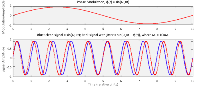
Figure 5: Adding phase-modulation (top curve) to a jitter-free signal (bottom blue curve) creates a jittered signal (bottom red curve). To observe one complete cycle of modulation on the jittered signal, the oscilloscope memory depth needs be large enough to capture 10 units of relative time in this example. If the waveform is acquired with 5 units of relative time, then only half of the modulation would be observed in the jittered signal.

Continuing the earlier measurements, Figure 2(d) shows how increasing the record length (i.e., memory depth) can increase the measured TIE values when lower-frequency noise is present in the signal or test environment. Notice also that period and C2C jitter remain constant with memory depth. This is because TIE jitter is, by definition, able to detect low-frequency noise, whereas period and C2C jitter, by definition, essentially filter out this low-frequency noise. Another consideration is that longer acquisitions of data increase the population of jitter data, which can statistically lead to higher peak values (even though this s ’ observed in Figure 2).

For TIE, the minimum required memory depth is the depth required to capture the lowest noise frequency pertaining to a specific application or standard. For example, if the application or standard requires TIE frequencies to be analyzed between 10 kHz and 20 MHz, and the oscilloscope requires 40 GSps to capture at least 5 samples per edge, then the minimum required memory depth is 40 GSps×10 kHz = 4 Mpts of data.

For period or C2C jitter, start with a small memory depth, then increase it until the value of jitter stays constant. To add a little margin, use a minimum memory depth slightly higher than this value. For Ncycle jitter, the minimum required memory depth is that needed to capture N continuous cycles.

Regardless of the type of jitter being measured, using the minimum required memory depth won't produce a large enough population to quantify jitter. The exact population depends on the application, but 1E+4 measurements is a good start for clock jitter (a lot more is needed for measuring jitter in data signals; refer to the high-speed data standard documentation). To increase the population of jitter measurements, increase the memory depth much higher than the required minimum value, or enable the measurement statistics to be accumulated over multiple acquisitions of data, or both.

10. Related resources

Refer to application note AN10007 Clock Jitter Definitions and Measurement Methods, for information on types of jitter, oscilloscope setup guidelines, and procedures on how to measure different types of jitter including period jitter, cycle-to-cycle jitter, and long-term jitter (i.e., N-cycle jitter).

Refer to AN10062 Phase Noise Measurement Guide for Oscillators for a theoretical overview of phase noise, recommended methods of phase noise measurement, and practical phase noise measurement guidelines for properly connecting a signal under test to the instrument, setting up the phase noise analyzer, and choosing appropriate settings.

Watch our Phase Noise Measurement Tutorial Video to learn how to achieve more accurate phase noise measurements using a phase noise analyzer. This tutorial includes tips on how to set up an analyzer, use the instrument features and settings, and how to interpret the results.

For more information on measuring jitter with a real-time oscilloscope when the level of jitter added to a signal from the measurement environment approaches or exceeds the signal's intrinsic jitter, refer to application note AN10074 Removing Oscilloscope Noise from RMS Jitter Measurements.

Table 1: Revision History