Contents
2.1.1 Period Jitter Applications
2.1.2 Calculating Peak to Peak Jitter from RMS Jitter"
2.1.3 Period Jitter Measurement Methodology
2.2.1 Cycle to Cycle Jitter Measurement Methodology
3 Jitter Measurements with a real time digital oscilloscope
3.1 Oscilloscope setup guidelines
3.1.1 Front-end amplifier noise
3.1.2 Quantization noise due to vertical gain setting
3.1.3 Quantization noise due to low sampling rate
3.2 Jitter measuring procedures using a real time digital scope
3.2.2 Measuring cycle-to-cycle jitter
3.2.3 Measuring long-term jitter
1. Introduction
Jitter is the timing variations of a set of signal edges from their ideal values. Jitters in clock signals are typically caused by noise or other disturbances in the system. Contributing factors include thermal noise, power supply variations, loading conditions, device noise, and interference coupled from nearby circuits.
2. Types of Jitter
Jitter can be measured in a number of ways; the following are the major types of jitter:
- Period Jitter
- Cycle to Cycle Period Jitter
- Long Term Jitter
- Phase Jitter
- Time Interval Error (TIE)
2.1 Period Jitter
Period jitter is the deviation in cycle time of a clock signal with respect to the ideal period over a number of randomly selected cycles. If we were given a number of individual clock periods, we can measure each one and calculate the average clock period as well as the standard deviation and the peak-to-peak value. The standard deviation and the peak-to-peak value are frequently referred to as the RMS value and the Pk-Pk period jitter, respectively.
Many publications defined period jitter as the difference between a measured clock period and the ideal period. In real world applications, it is often difficult to quantify the ideal period. If we observe the output from an oscillator set to 100 MHz using an oscilloscope, the average measured clock period may be 9.998 ns instead of 10 ns. So it is usually more practical to treat the average period as the ideal period.
2.1.1 Period Jitter Applications
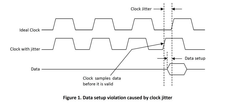
Period jitter is useful in calculating timing margins in digital systems. Consider a microprocessor-based system in which the processor requires 1 ns of data setup before clock rise. If the period jitter of the clock is -1.5 ns, then the rising edge of the clock could occur before the data is valid. Hence the microprocessor will be presented with incorrect data. This example is illustrated in Figure 1.
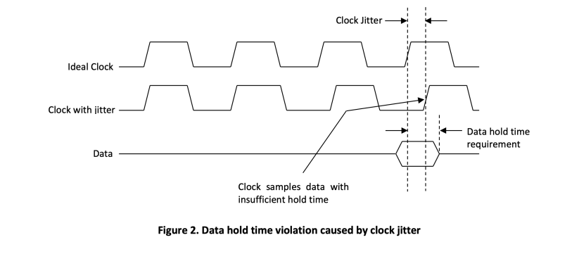
Similarly, if another microprocessor has a data hold time requirement of 2 ns but now the clock jitter is +1.5 ns, then the data hold time is effectively reduced to 0.5 ns. Once again, the microprocessor will see incorrect data. This situation is illustrated in Figure 2.
2.1.2 Calculating Peak to Peak Jitter from RMS Jitter
Because the period jitter from a clock is random in nature with Gaussian distribution, it can be completely expressed in terms of its Root Mean Square (RMS) value in pico-seconds (ps). However, the peak-to-peak value is more relevant in calculating setup and hold time budgets. To convert the RMS jitter to peak-to-peak (Pk-Pk) jitter for a sample size of 10,000, the reader can use the following equation:
𝑃𝑒𝑎𝑘‒ 𝑡𝑜‒ 𝑝𝑒𝑎𝑘 𝑝𝑒𝑟𝑖𝑜𝑑 𝑗𝑖𝑡𝑡𝑒𝑟 = ±3.719 𝑥 (𝑅𝑀𝑆 𝑗𝑖𝑡𝑡𝑒𝑟) Equation 1
For example, if the RMS jitter is 3 ps, the peak to peak jitter is ±11.16 ps.
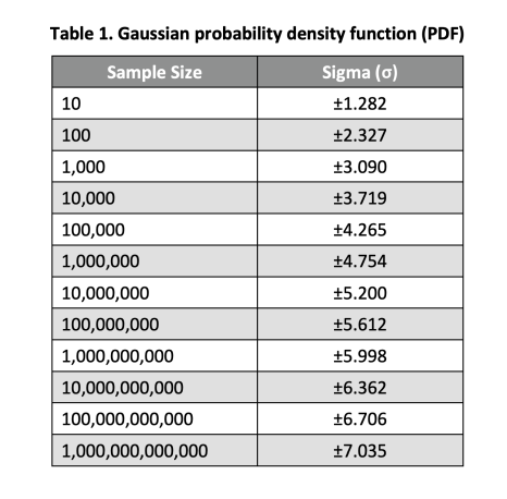
Equation 1 is derived from the Gaussian probability density function (PDF) table. For instance, if the sample size is 100, 99 of those samples will fall within ±2.327σ from the mean value of the distribution, only 1 sample, on average, will fall outside that region. SiTime measures the RMS period jitter over a sample size of 10,000 as specified by the JEDEC standard.
2.1.3 Period Jitter Measurement Methodology
Period Jitter is defined in JEDEC Standard 65B as the deviation in cycle time of a signal with respect to the ideal period over a number of randomly selected cycles. The JEDEC standard further specified that period jitter should be measured over a sample of 10,000 cycles. SiTime recommends measuring period jitter using the following procedure:
- Measure the duration (rising edge to rising edge) of one clock cycle
- Wait a random number of clock cycles
- Repeat the above steps 10,000 times
- Compute the mean, standard deviation (σ), and the peak-to-peak values from the 10,000 samples
- Repeat the above measurements 25 times. From the 25 sets of results, compute the average peak-to-peak value.
The standard deviation (σ) or RMS value computed from a measurement of 10,000 random samples(step 4) is quite accurate. The error in the RMS value can be calculated using the following equation:

where σn is the RMS (or sigma) of the collected sample and N is the sample size. For a sample size of 10,000, ErrorRMS is 0.0071σn. This error is random and it follows the Gaussian distribution. The worst-case measurement error is typically computed as ±3 ErrorRMS.
For example, if the RMS value computed from 10,000 random samples is 10 ps, then the ErrorRMS will be 0.071 ps and virtually all the RMS values of this measurement will still fall within a narrow range of 10 ± 0.213 ps. In practical applications, the RMS errors in a sample set of 10,000 are small enough to be ignored.
While an accurate RMS value can be computed from a random 10000-sample set, the peak-to-peak value is more difficult to measure. Due to the random nature of period jitter, the larger the sample size, the higher is the probability of picking up data points at the far ends of the distribution curve. In other words, the peak-to-peak value diverges instead of converging as more samples are collected. That is the reason why we added an extra step, step 5 to produce a more consistent and repeatable peak-to-peak measurement.
Each measurement of 10,000 random samples (step 4) produces one standard deviation value and one peak-to-peak value. By randomly repeating this process 25 times, we could collect a good set of data points from which we can calculate the average peak-to-peak value with a high degree of accuracy. We can also compute the average RMS value from this data, but it will be very close to the RMS value derived from each individual run.
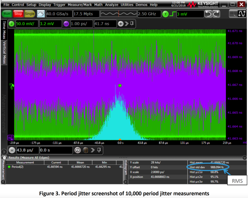
Figure 3 is the period jitter histogram and period trend of a 3.3V TCXO oscillator running at 24 MHz captured by DSA90804A Infiniium High Performance Oscilloscope. It represents one set of RMS value measured from 10,000 samples (step 4).
2.2 Cycle to Cycle Jitter
Cycle to cycle (C2C) jitter is defined in JEDEC Standard 65B as the variation in cycle time of a signal between adjacent cycles, over a random sample of adjacent cycle pairs. The JEDEC standard further specified that each sample size should be greater than or equal to 1,000. Please note that cycle to cycle jitter only involves the difference in period between 2 consecutive cycles, there is no reference to an ideal cycle.
Cycle to cycle jitter is typically reported as a peak value in ps which defines the maximum deviation between the rising edges of any two consecutive clocks. This type of jitter specification is commonly used to illustrate the stability of spread spectrum clocks because the period jitter is more sensitive to the frequency spreading feature while C2C jitter is not. Cycle to cycle jitter is sometimes expressed as a RMS value in ps as well.
2.2.1 Cycle to Cycle Jitter Measurement Methodology
SiTime recommends measuring cycle to cycle jitter using the following procedure:
- Measure the cycle times of two adjacent clock cycles, T1 and T2
- Calculate the value of T1-T2. Record the absolute value of this number.
- Wait a random number of clock cycles
- Repeat the above steps 1,000 times
- Compute the standard deviation (σ), and the peak value from the 1,000 samples. The peak value is the largest absolute (T1-T2) number in the data set.
- Repeat above measurements 25 times and calculate the average peak value from the 25 sets of results.
Similar to the peak-to-peak period jitter, the peak value of the cycle to cycle jitter also diverges instead of converging as more samples are taken. Step 6 in the procedure is added to obtain the average peak C2C jitter from 25 sample sets.
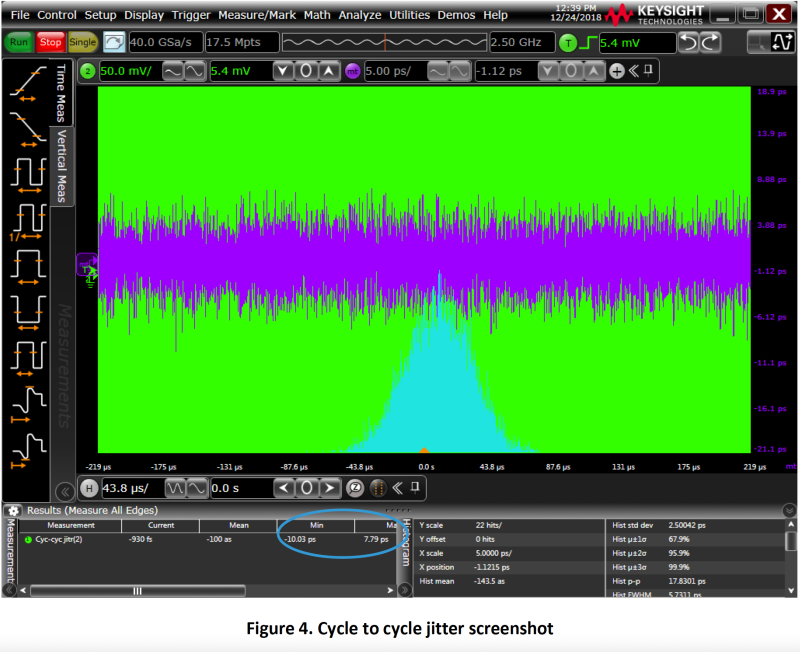
Figure 4 is an example of the cycle to cycle jitter histogram and period trend. In this case, the peak cycle to cycle jitter is 10.03 ps (the bigger of the two numbers: -10.03 ps and 7.79 ps expressed in the absolute form).
2.3 Long-Term Jitter
Long-term jitter measures the change in a clock’s output from the ideal position, over several consecutive cycles. The actual number of cycles used in the measurement is application dependent. Long-term jitter is different from period jitter and cycle-to-cycle jitter because it represents the cumulative effect of jitter on a continuous stream of clock cycles over a long time interval. That is why long-term jitter is sometimes referred to as the accumulated jitter. Long-term jitter is typically useful in graphics/video displays and long-range telemetry applications such as range finders.
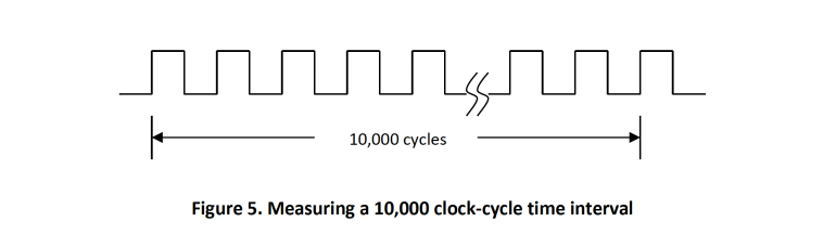
SiTime recommends measuring long-term jitter using the following method; in this example, we measure the long-term jitter over 10,000 clocks.
- Measure the time interval of 10,000 consecutive clock cycles as shown in Figure 5
- Wait a random number of clock cycles
- Repeat the above steps 1,000 times
- Compute the mean, standard deviation (σ), and the peak-to-peak values from the 1,000 samples
- Repeat above measurements 25 times. From the 25 sets of results, compute the average peakto-peak value.
Once again, step 5 is needed to overcome the un-bounded nature of the peak-to-peak value.
2.4 Phase Jitter
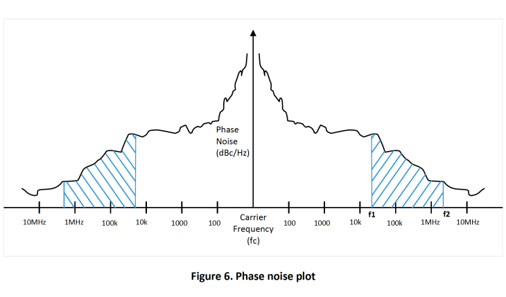
Phase noise is usually described as either a set of noise values at different frequency offsets (e.g., -60 dBc/Hz at 20 kHz and -95 dBc/Hz at 10 MHz), or as a continuous noise plot over a range of frequencies. Phase jitter is the integration of phase noises over a certain spectrum and expressed in seconds.
In a square wave, most of the energies are located at the carrier frequency. However, some signal energies are “leaked-out” over a range of frequencies on both sides of the carrier. Phase jitter is the amount of phase noise energy contained between two offset frequencies relative to the carrier (fc). Figure 6 is an unfiltered phase noise plot and the shaded areas represent the phase jitter between frequencies f1 and f2.
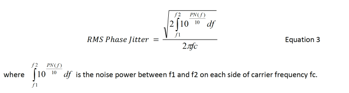
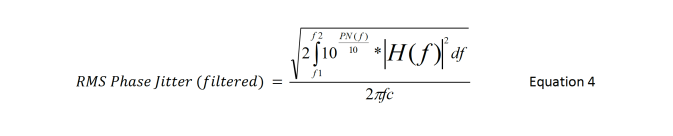
The RMS phase jitter between f1 and f2 is defined by Equation 3.
In communication applications, the bandpass filter effect of the combined TX PLL and RX PLL is applied to the raw phase noise data before the final RMS phase jitter value is calculated. The following are common applications and the bandwidth (corner frequencies) of their associated filters:
- SONET OC-48: 12 kHz to 20 MHz
- Fibre Channel: 637 kHz to 10 MHz
- SATA/SAS: 900 kHz to 7.5 MHz
- 10 Gigabit Ethernet XAUI: 1.875 MHz to 20 MHz
If the filter function is H(f), then the filtered RMS phase jitter can be calculated using Equation 4.
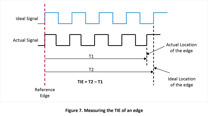
2.5 Time Interval Error (TIE)
Time Interval Error (TIE) of an edge is the time deviation of that edge from its ideal position measured from a reference point. In effect, TIE is the discrete time domain representation of phase noise expressed in seconds or pico-seconds. Figure 7 illustrates the basic concept of TIE. The ideal signal is often a signal created in software from an average estimate of the signal period.
2.5.1 Plotting TIE over time
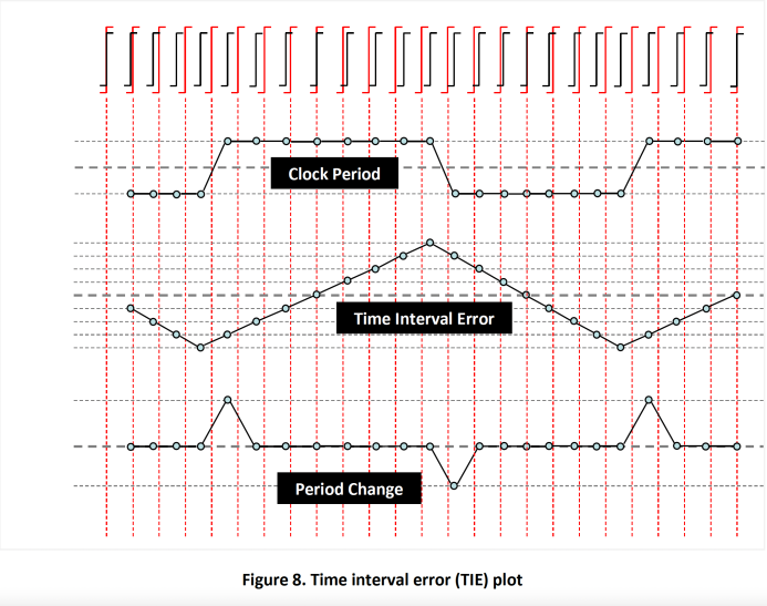
A clock waveform is shown at the top of Figure 8. The red pulses are perfectly timed clock cycles exactly 1000 ps in duration. The pulses in black are clock cycles with jitter. The trailing edges of these clock pulses have been removed to enhance the presentation. At the beginning of the sequence, both the red and black clocks are aligned to each other. Because of the jitter, the black clock edges will start shifting in time, sometimes occurring before the red clock edge and sometimes after.
The plot labeled “Clock Period” represents the measured black clock periods over time. In this example, the black clock periods are either 990 ps or 1010 ps. The “Period Change” plot depicts each cycle’s change from the previous cycle. This graph remains flat as long as the period between two consecutive black clocks stays the same. However, it will register a change whenever a period difference is detected.
For example, the period of the first 4 clock cycles are constant at 990 ps, so the “Period Change” plot is flat; but when the period of the fifth clock is lengthened from 990 ps to 1010 ps, the plot reports this change by jumping to the +20 ps position. In other words, this plot identifies the period changes shown in the “Clock Period” plot.
The “Time Interval Error” (TIE) plot documents the accumulated error between the ideal edge (red clock) and the actual edge (black clock). In this example, the TIE plot begins by moving towards the negative direction because the first 4 clocks are each 10 ns shorter than the ideal period. After accumulating -40 ps in jitter error, the plot changes direction at the fifth clock and heads towards the positive direction because the fifth clock period is 10 ps longer than the ideal period.
TIE measurements are especially useful when examining the behavior of transmitted data streams, where the reference clock is typically recovered from the data signal using a Clock/Data Recovery (CDR) circuit. A large TIE value may indicate that the PLL in the CDR is too slow in responding to the data stream’s changing bit rate.
3. Jitter Measurements with a real time digital oscilloscope
3.1 Oscilloscope setup guidelines
The most common instrument used in measuring clock jitter is the real time digital oscilloscope (scope). This section contains general scope setup guidelines to yield better jitter measurement accuracy.
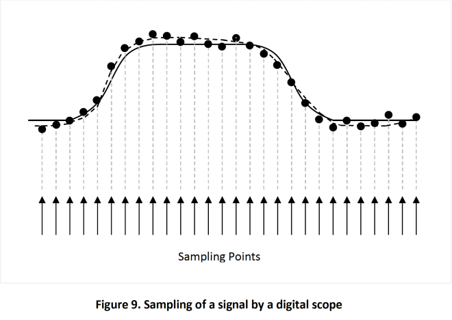
The digital scope uses an internal time base to sample its inputs at regular intervals. The sampling rate can range from 1 Gsps (giga-samples-per-second) to 40 Gsps for the high-end units. Figure 9 illustrates how the digital scope samples and displays a signal presented to its inputs. The arrows at the bottom of the figure represent the sampling points, the solid line is the actual signal, and the dots are the sampled values. The signal displayed by the scope (represented by the dotted line) is the best-fit curve across the sampled points.
The reader may notice that the sampled values do not always match that of the actual signal. These discrepancies are caused by quantization errors in the scope. Most of these errors are inherent in the design/cost tradeoffs of the scope but proper scope setup can mitigate some of the inaccuracies. In the following sections, we will explore the main causes of these errors and recommend steps to reduce their impact on jitter measurements.
3.1.1 Front-end amplifier noise
The inputs to a digital scope passed through an analog amplifier before they are digitized by the Analog to Digital Converter (ADC). The noise produced by this amplifier is proportional to the input bandwidth of the scope: the wider the bandwidth, the higher the noise. However, reducing the bandwidth too much will affect the rising and fall time of the sampled signal, thus introducing significant errors to the jitter measurement.
The general equation describing the relationship between rise time/fall time and the bandwidth of the signal edge is:

where the rise time (or fall time) is measured between the 20% and the 80% points of the signal edge. SiTime recommends setting the scope bandwidth to 3 times the bandwidth of the signal. In some scopes, the bandwidth can be set only if the maximum sampling rate is selected. In other scopes, the bandwidth may not be selectable at all.
3.1.2 Quantization noise due to vertical gain setting
Quantization error is the difference between the sampled value and the actual value of the signal at the sampling point. This error is shown in Figure 9. A portion of this error in a scope is caused by the vertical gain setting of the display. If the vertical gain is set to small value, the scope may not utilize the full resolution of its internal ADC.
SiTime recommends adjusting the vertical gain control of the scope until the signal fills the entire height of the display. In some scopes, turning the vertical gain up an additional notch so that a small portion of the signal is clipped at both the top and bottom of the display could further reduce the quantization error. This benefit is achieved because the higher vertical gain setting may cause the scope to utilize an extra bit in the ADC to digitize the signal. However, this feature is scope dependent, so please consult your scope manual.
3.1.3 Quantization noise due to low sampling rate
Some of the quantization noise described in the previous section is caused by insufficient sampling points along the horizontal axis. SiTime recommends having at least 3 sampling points falling between the 20% and 80% points of a rising or falling edge. This recommendation translates into a minimum sampling rate requirement for the scope. For example, if rise time (20% - 80%) of a signal is 1 ns and 4 sampling points are needed within this time frame, then the scope must have a sampling rate better than 4 Gsps. If your scope has a higher sampling rate than the minimum requirement specified above, select the highest sampling setting.
3.1.4 Time base jitter
The sampling points in a digital scope are generated by an internal time base. As a clock source, the time base has its own jitter characteristics and it will contribute to the jitter measurement error of a signal. Generally speaking, time base jitter should be kept below 25% of the of the expected signal jitter to support jitter measurement with better than 3% accuracy. SiTime recommends using the best scope available in your laboratory to perform jitter measurements because higher end units tend to have better time base circuits with lower jitter.
3.2 Jitter measuring procedures using a real time digital scope
3.2.1 Measuring period jitter
Method A
- Configure the scope to measure all the sampled clock periods instead of just measuring the first clock.
- Configure the scope to capture 10,000 clock cycles on the screen. For example, for a 100 MHz clock, 10K cycles = 100 us. Since the display usually contains 10 horizontal divisions, the horizontal control should be set to 10 us per division.
- Record the mean, the standard deviation, and the peak-to-peak values reported by the scope.
- The mean and standard deviation values are quite accurate. The peak-to-peak value, however, is not very accurate due to its unbounded nature (see section 2.1.3). Follow the next step to obtain a more accurate peak-to-peak value.
- Repeat steps 2 and 3 twenty five (25) times. Record the peak-to-peak value after each run and compute the average peak-to-peak value from the 25 results.
Method B (the JEDEC method)
- Configure the scope to measure the period of the first clock and turn on the histogram feature, if available.
- Configure the scope to capture a single clock cycle on the screen.
- Repeat the above step 10,000 times.
- Record the mean, the standard deviation, and the peak-to-peak values reported by the scope.
- The mean and standard deviation values are quite accurate. The peak-to-peak value, however, is not very accurate due to its unbounded nature (see section 2.1.3). Follow the next step to obtain a more accurate peak-to-peak value.
- Repeat steps 2 through 4 twenty five (25) times. Record the peak-to-peak value after each run and compute the average peak-to-peak value from the 25 results.
3.2.2 Measuring cycle-to-cycle jitter
- Turn on the histogram feature in your scope, if available.
- Turn on the C2C feature in your scope. If this feature is not available, configure the scope to capture two consecutive clock cycles on the screen; subtract the period of the second clock from the period of the first clock and record the absolute value of the difference.
- Repeat the above step 1,000 times.
- If the scope has the histogram feature, record the standard deviation and the peak value. If the histogram feature is not available, compute the standard deviation and the peak value from the 1000 data sets. The peak value is the biggest difference between any two consecutive clocks in the data set.
- The standard deviation value is quite accurate. The peak value, however, is not very accurate due to its unbounded nature (see section 2.1.3). Follow the next step to obtain a more accurate peak value.
- Repeat steps 2 through 5 twenty five (25) times. Record the peak value after each run and compute the average peak value.
3.2.3 Measuring long-term jitter
Method A
- Configure the scope to capture N+1 clock cycles on the screen. N is your definition of the number of clock cycles needed in the long-term jitter measurement.
- Set the scope to measure the time between the rising edge of the first clock and the rising edge of clock N+1.
- Repeat the above steps 1,000 times
- Calculate the mean, the standard deviation, and the peak-to-peak values from the 1,000 samples
- The mean and standard deviation values are quite accurate. The peak-to-peak value, however, is not very accurate due to its unbounded nature (see section 2.1.3). Follow the next step to obtain a more accurate peak-to-peak value.
- Repeat steps 1 through 4 twenty five (25) times. Record the peak-to-peak value after each run and compute the average peak-to-peak value.
Method B
- Configure the scope to display the rising edge of a clock cycle on the screen.
- Assuming that the long-term jitter measurement involves N clock cycles each with a period of T ns. Set the scope to trigger N*T ns before the displayed edge.
- Turn on the histogram mode to capture the 50% crossing of the waveform 1,000 or 10,000 times, as the application requires. In some scope, this may require defining vertical and horizontal thresholds for the edge detection; please refer to your scope manual.
- Wait until the target number of hits is recorded in the histogram. Stop the acquisition as soon as the target number is reached.
- The screen will show the rising edge as a band of lines (see Figure 10) and the width of the band is the long-term jitter.
- Record the mean, the standard deviation, and the peak-to-peak values from the scope.
- The mean and standard deviation values are quite accurate. The peak-to-peak value, however, is not very accurate due to its unbounded nature (see section 2.1.3). Follow the next step to obtain a more accurate peak to peak value.
- Repeat steps 3 through 4 twenty five (25) times. Record the peak-to-peak value after each run and compute the average peak-to-peak value.

4. Conclusion
This application note serves two purposes. First, it describes the common types of jitter that the reader may encounter in today’s high speed systems. Second, it provides the procedures to capture the various types of jitters using a real time digital oscilloscope. Phase noise and consequently phase jitter measurement technique is described in the AN10062 Phase Noise Measurement Guide for Oscillators.