Content
2 Probing on SiTime Evaluation Board
3.1 Probe influence on the signal under test
3.2 Long wires and ground lead inductance
3.3 Examples of good probing practices
4.1 Bandwidth and input capacitance of the probe are not appropriate
4.2 Long wires used for probing
4.3 Stubs connected to the signal under test
4.4 Oscilloscope sample rate is too low
1 Introduction
Electrical engineers often use oscilloscopes for purposes ranging from checking simple, low-speed digital signals to accurate waveform and jitter measurements. They need to use probes to directly access arbitrary signals on a PCB. Probes can, however, put extra load on a signal or distort the waveform displayed on a scope. Therefore, probing should be done carefully.
This application note gives practical guidelines for the effective probing of oscillator output, shows common mistakes and explains how to identify and avoid potential probing issues.
2 Probing on SiTime Evaluation Board
Evaluation boards are great tools for testing the performance of an oscillator. They are carefully designed, tested and have dedicated test points for probing. Nevertheless, evaluation results may be inaccurate because of improper probing or measurement techniques.
Figure 2.1 illustrates waveform measurements of a SiT8208 10 MHz MEMS oscillator soldered onto a SiTime evaluation board. Ideal measurement with a 1.5 GHz bandwidth and <1 pF capacitance active probe is compared to measurements with a 10 MΩ input impedance, 16 pF capacitance passive probe using two ground connection options. Rise time measured with a passive probe is larger than that measured with an active probe. Figure 2.1 also shows that the ground wire of a passive probe causes ringing, over- and undershoots and further increases rise time.
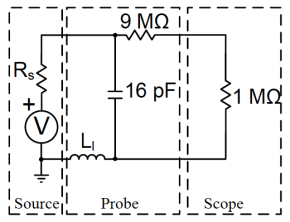
The model of a passive probe (Figure 2.2) explains the measurement results. Self-inductance of a ground loop ( ) depends on the area of the loop and in our example is 200 nH. Together with 16 pF input capacitance and 25 Ω oscillator output resistance ( ) it forms a loop with 13-dB resonance at about 90 MHz. That resonance causes excessive ringing after fast rising or falling edges. Removing the ground wire and touching the SMA with the probe collar reduces by reducing the ground wire loop area and thus eliminates ringing. l L s R l L
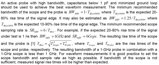
Frequency response of the probe input model has a -40 dB per decade roll-off after resonance frequency, so increasing ground loop self-inductance limits probe bandwidth. This is essential since measured rise time of a signal is calculated as below [1]

where TScope, TProbe, and TSignal are the rise times of the scope, probe and signal, respectively. This explains why rise time measured with a low bandwidth passive probe is higher than with a 1.5-GHz active probe. Scope T obe TPr Signal T
Active probes solve many issues that are encountered with passive probes. Active probes are high bandwidth and typically have input capacitance below 1 pF. Advanced grounding accessories are designed for active probes that help minimize size of the ground loop. Also, since input capacitance of an active probe is typically much lower than input capacitance of a passive probe it shows less resonance for the same ground loop size.
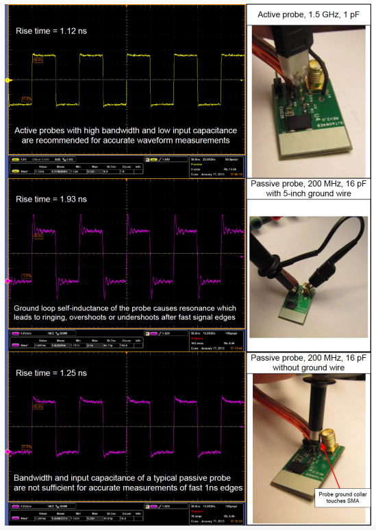
Figure 2.1: Probing on an evaluation board: Tektronix DPO7104 1-GHz oscilloscope using active probe, passive probe with ground loop, and passive probe without ground loop
3 In-System Probing
Debugging and performance verification are common stages in product design. They involve measuring various signals in the system and require accurate oscilloscope measurements, so close attention should be paid to probing techniques.
3.1 Probe influence on the signal under test
Every probe functions as an external circuit connected to the test point. It has its own input capacitance and resistance and thus imposes additional load on the circuit. It is therefore important to consider the influence of active and passive probes on the signal under test.
3.1.1 Active probes
Active probes are usually high bandwidth, have low input capacitance and are the preferable choice for probing clock signals. Input capacitance of active probes ranges from 0.3 pF to 8 pF. A typical oscillator has a 15 pF output load rating, so selecting an active probe with 1 pF or less input capacitance is recommended.
Input resistance of active probes varies from 30 kΩ to 10 MΩ depending on the probe model. SiTime oscillators have significantly lower output impedance, so this range of probe resistances is acceptable for measuring output waveforms. Input resistance can, however, be a significant factor when probing high impedance sources.
3.1.2 Passive probes
Passive probes having 100 to 300 MHz bandwidth and 10 to 17 pF input capacitance are most common. Such probes impose excessive load on the oscillator output. For example, if the in-system load of the oscillator output is 12 pF then using a passive probe with 12 pF input capacitance doubles the load. The new load of 24 pF exceeds the 15 pF oscillator load rating. Output parameters, especially rise time, measured with such a probe may not meet datasheet specifications. Figure 3.1 illustrates how the oscillator output signal is affected by a 16 pF passive probe.
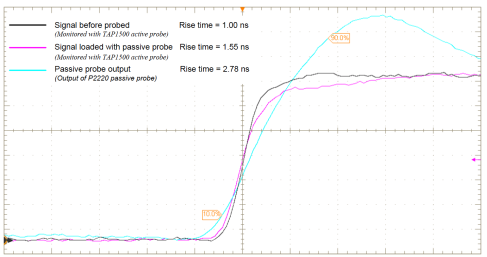
Figure 3.1: Impact of 16 pF passive probe input capacitance on the signal under test. Test signal is monitored with a high performance active probe before and after connecting a passive probe. Captures made with Tektronix DPO7104 1-GHz oscilloscope.
The most popular types of passive probes have either 1 MΩ or 10 MΩ input resistance specified in the datasheet. These passive probes are intended to use only with 1-MΩ oscilloscope input, and the resistance specified for the probe already takes into account the 1-MΩ scope termination. This means that the resistance of a 10-MΩ probe is 9 MΩ, as shown in Figure 2.1. When connected to a 1-MΩ scope input the full resistance of the loop is 10 MΩ and the resulting voltage divide ratio is 10:1.
If a 10-MΩ probe is connected to a 50-Ω scope input, no signal will be visible on the scope. The 50-Ω scope termination and 9 MΩ probe resistance form a voltage divider that attenuates input to the scope amplifier beyond the measurable limit.
3.2 Long wires and ground lead inductance
Finding a ground connection point close to the measurement point may be difficult, so a long wire is sometimes used to reach the most convenient ground terminal. This creates a large ground loop, which causes ringing and over- or undershoots after fast signal edges, as discussed in section 2. Figure 3.2 uses a passive probe to illustrate the impact of ground wire length on a waveform measurement. Using lower input capacitance probe reduces resonance. Figure 3.3 illustrates that a ground wire of the same length used with a 1-pF active probe has much less effect on the waveform.
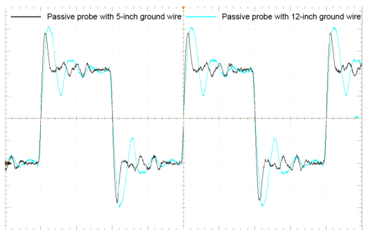
Figure 3.2: Ground wire length impact on the waveform measurements with passive probe. Longer ground wire increases ringing after fast signal edges. Oscilloscope: Tektronix DPO7104. Passive probe: Tektronix P2220 in 10 MΩ mode connected to 1 MΩ input.
During high and low temperature testing, engineers find it convenient to connect a probe using extension wires. Such an approach has several drawbacks, including noise pickup from the neighboring circuits (see Section 3.4), and large self-inductance of the loop which leads to reduced bandwidth, ringing, over- or undershoots. The area of the loop changes when the wires are moved, which changes the shape of the waveform. Figure 3.4 illustrates waveforms captured using 22-inch wires with two different wire positions, showing significant overshoots and undershoots. If the signal frequency is close to wire/probe resonance frequency, the waveform may appear as sine-wave with amplitude exceeding the power supply rails.
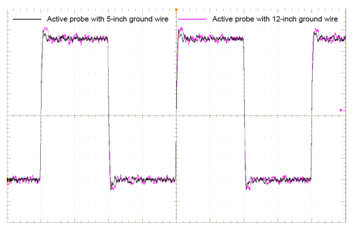
Figure 3.3: Ground wire length impact on the waveform measurement with 1-pF active probe. Low capacitance active probe is less sensitive to ground wire length. Oscilloscope: Tektronix DPO7104. Active probe: Tektronix TAP1500.
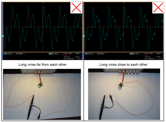
Figure 3.4: Probing 10 MHz signal under test with 22-inch wires and Tektronix P2220 passive probe in 10 MΩ mode connected to 1 MΩ Tektronix DPO7104 oscilloscope input.
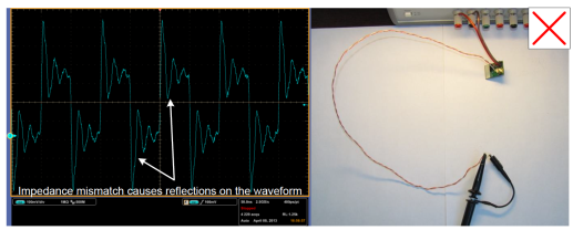
Figure 3.5: Probing 10 MHz signal under test with 22-inch twisted pair and Tektronix P2220 passive probe in 10 MΩ mode connected to 1 MΩ Tektronix DPO7104 oscilloscope input.
Self-inductance of the wires can be minimized using a transmission line structure, for example a twisted pair as shown in Figure 3.5. Impedance of such hand-made transmission lines is hard to predict and may vary along the line, causing impedance mismatch. The signal travelling through the transmission line reflects from every point of impedance change, including the probe connection point. Reflections are superimposed with the signal and thus distort the measured waveform. To reduce reflections 50-Ω resistor between signal and ground may be used as load termination at the probe-to-wires connection point (Figure 3.6). Another 20-Ω resistor in series with the DUT output may be used for better source impedance matching and output current reduction. Since signal integrity issues in twisted pair transmission line approach are very hard to eliminate this method is not recommended for probing.
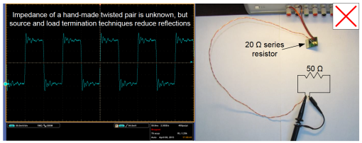
Figure 3.6: Probing 10 MHz signal under test with 22-inch twisted pair and Tektronix P2220 passive probe in 10 MΩ mode connected to 1 MΩ Tektronix DPO7104 oscilloscope input. Source and load termination techniques used to reduce reflections.
Another possible solution is using a 50-Ω coaxial cable connected directly to the 50-Ω instrument input. A series termination resistor should be placed close to the oscillator output for impedance matching. It also provides some isolation of the coaxial cable capacitance from the oscillator output driver. Typical output impedance of a standard SiTime single-ended oscillator is about 20 to 30 Ω for 2.5, 2.8, 3.0 or 3.3 V supply voltages and 25 to 35 Ω for 1.8-V oscillators. Thus a series termination resistor with a value between 20 and 30 Ω is recommended, as shown in Figure 3.7. Source impedance (Zs ) and load termination (Zt ) form a voltage divider with a (Zs + Zt)/Zt : 1 ratio. Output impedance of the oscillator depends on output driver properties and can also vary with external conditions, such as temperature. Therefore, the voltage divider ratio is not precise and this approach should not be used for voltage measurements. It is better suited for frequency testing with the oscilloscope, frequency counter (as shown on figure 3.8) or any other instrument. Regardless of instrument choice, either an external or built-in 50-Ω termination is required at instrument side. Also, note that this method imposes an extra 70-Ω resistive load on the oscillator output.
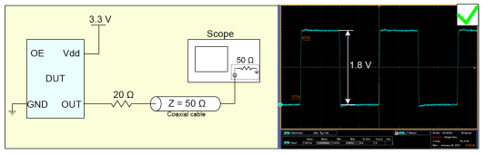
Figure 3.7: Probing oscillator output with 50-Ω coaxial cable (approximately 2:1 divide ratio)
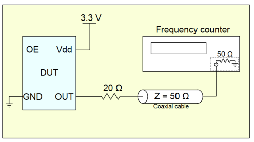
Figure 3.8: Connecting frequency counter using 50-Ω coaxial cable
Another probing scheme that may be used with coaxial cable is shown in Figure 3.9. It has higher input impedance, a divide ratio of about 21:1, and isolates the oscillator output from the coaxial cable with a 1-kΩ resistor. Since the scope termination resistance is very accurate and oscillator output impedance is fairly low, accuracy of the divide ratio mostly depends on the 1-kΩ resistor. The drawback of this method is a high attenuation factor, which places additional demands on the scope input amplifier.
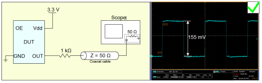
Figure 3.9: Probing oscillator output with 50-Ω coaxial cable (21:1 divide ratio)
3.3 Examples of good probing practices
The recommended gain of the scope vertical amplifier is one that stretches the input signal as much as possible, so long as it still fits on the screen. This ensures that the maximum resolution of the scope ADC is utilized for waveform conversion so quantization noise is minimized. The auto set feature of the scope usually selects the optimum vertical resolution for the waveform capture. Figure 3.10 shows a good probing example of 75-MHz oscillator output.
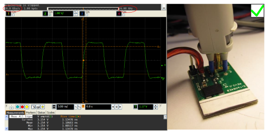
Figure 3.10: Probing example. Signal source: 75-MHz SiT8208 MEMS oscillator on SiTime evaluation board. Oscilloscope: Agilent DSA90604A (6 GHz). Active probe: Agilent 1134A (7 GHz) with E2675A differential browser probe head.
An active probe cannot be placed into the temperature chamber since its operating temperature range is fairly narrow. For example, an Agilent 1169A active probe operates between 5 and 40 °C. A typical setup with extension cables is illustrated in Figure 3.11. If these accessories are not available, then coaxial cabl e may be used for some measurements, such as frequency testing, as discussed in section 3.2. Figure 3.12 shows a typical measurement configuration using coaxial cable.
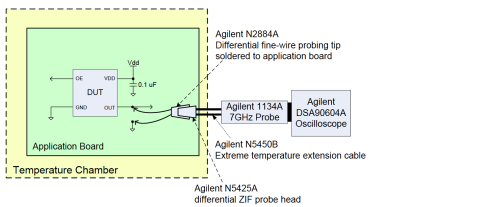
Figure 3.11: Example of a temperature testing setup that utilizes Agilent temperature extension cable
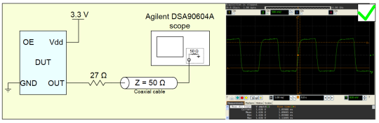
Figure 3.12: Probing with Agilent DSA90604A scope using coaxial cable
3.4 Noise pick-up
The probe ground loop picks up noise from various sources on the applications board. This coupled noise shows up on the waveform, as if it has been naturally present on a signal under test. If noise comes from a source synchronous with the oscillator it is hard to separate it from the native signal noise.
Figure 3.13 shows the mechanism of the noise coupling to the probe ground loop. Switching current signal travelling along a trace on the board forms a loop with the ground return current. It couples to the probe ground loop through mutual inductance of two loops. Amplitude of the coupled noise depends on the rate of disturbing current change and mutual inductance between the loops. Mutual inductance is proportional to the loop areas and inversely proportional to the cube of distance between the lo ops. To minimize noise pickup it’s recommended to keep the area of a probe ground loop as small as possible.
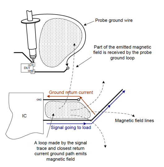
Figure 3.13: Mechanism of noise coupling to the probe ground loop
3.5 Probing tips
As mentioned above, active probes are recommended for probing oscillator output. Passive probes are, however, useful in certain situations.
Passive probes are recommended for:
- Debugging low speed digital circuits
- Low bandwidth analog circuits
- Low speed, high impedance sources
- Probing DC sources
Active probes are recommended for:
- Probing high speed serial interfaces
- Clock waveform measurements
- Probing high frequency digital circuits
4 Common Mistakes
4.1 Bandwidth and input capacitance of the probe are not appropriate
Figure 4.1 shows a 75-MHz waveform captured with a Tektronix P2220 passive probe switched to ”1X” mode. In this mode the P2220 probe has 95 pF input capacitance and only 6-MHz bandwidth. The waveform in Figure 6.1 doesn’t reach its full swing and has slow rise times.
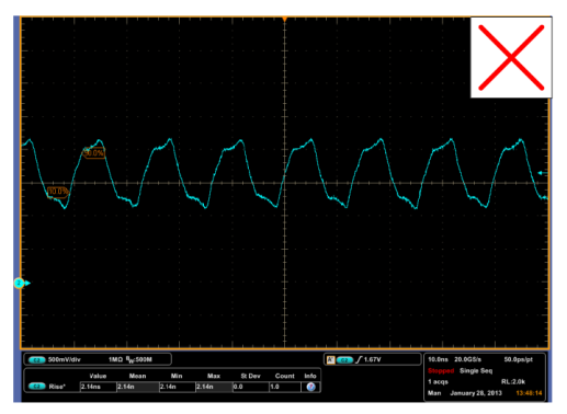
Figure 4.1: 75-MHz oscillator output captured with a Tektronix P2220 passive probe in ”1X” mode on Tektronix DPO7104 scope
4.2 Long wires used for probing
Figure 4.2 illustrates a 75-MHz oscillator output waveform captured using 22-inch wires and a 10-MΩ passive probe. Loop self-inductance of the long wires causes resonance and bandwidth reduction.
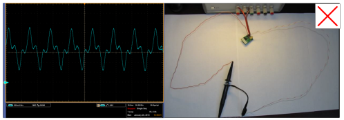
Figure 4.2: Probing using long wires and a Tektronix P2220 10-MΩ passive probe. Screen capture made with Tektronix DPO7104 oscilloscope.
Any wires or PCB traces on the signal path that are longer than one-sixth of the effective rising edge length in the material are treated as the transmission line with distributed parameters and require impedance matching. For a signal with a 1 ns rise time, this threshold is about 1 inch. As a result, there are significant reflections when non-terminated transmission lines or long wires are connected to a 10-MΩ passive probe. Signal travelling through the line shown in Figure 4.2 reflects from the high impedance input of the probe and since there is no proper source termination, the reflected wave reaches source and reflects back.
4.3 Stubs connected to the signal under test
Any long stubs connected to the signal under test cause reflections. Figure 4.3 shows the waveform captured on the evaluation board using a 6-GHz active probe, but with a 4-ft coaxial cable connected to the signal trace. The other end of the 50-Ω coaxial cable is floating, so impedance mismatch causes reflections.
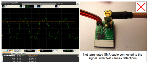
Figure 4.3: Waveform captured on evaluation board with an active probe while a non- terminated coaxial cable is connected to the oscillator output. Oscilloscope: Agilent DSA90604A (6 GHz); active probe: Agilent 1134A (7 GHz) with E2675A differential browser probe head.
4.4 Oscilloscope sample rate is too low
Improper sample rate selection can lead to unexpected waveforms appearing on the scope screen and therefore may be mistaken for a probing issue. Figure 4.5 illustrates a 75-MHz signal captured using two sampling rates (25 Msps and 50 Msps) that are both lower than the Nyquist frequency for the first harmonic (150 MHz). Such a situation is most often encountered when attempting to capture a rather large time frame of the signal, causing the oscilloscope to automatically reduce the sampling rate due to limited memory. Aliasing appears in the under-sampled signal, which makes high frequency components look like low frequency components. With this low sampling rate neither of the captured waveforms looks like a 75 MHz clock signal. The waveform displayed on the scope may look like a very low frequency signal or gaps in the waveform may appear. This may lead to the incorrect assumption that the oscillator is not functioning properly.
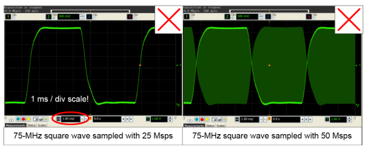
Figure 4.5: 75-MHz signal under test captured with Agilent DSA90604A scope using the sampling rates below the Nyquist frequency.
5 References
[1] Howard W. Johnson, Martin Graham. High-speed digital design: a handbook of black magic. Upper Saddle River, New Jersey: Prentice Hall PTR, 1993, pp. 83-101
[2] Agilent technologies. Application note 1603, “Eight hints for better scope probing” (http://cp.literature.agilent.com/litweb/pdf/5989-7894EN.pdf) (2011).
[3] Tektronix. Primer, “ABCs of Probes” (http://www.tek.com/document/primer/abcs-probes)
[4] LeCroy. Application note 016, “Probing tutorial” (http://cdn.teledynelecroy.com/files/appnotes/lecroy_probing_tutorial_appnote016.pdf)